How does plasma shape enter a stability calculation?
A plasma can lose stability in several different ways. CHIHIRO studies how geometry enters the equations for those disturbances—and how to keep the resulting diagnostics connected to their assumptions.
Start with the shape. Then specify the disturbance.
Magnetic fields hold the plasma in a toroidal configuration. Its cross-section can be circular, stretched vertically, or bent into a D-like shape. Those choices enter the stability operator: the mathematical model that asks whether a small disturbance grows.
The work follows that question through shaped ballooning calculations, self-consistent equilibrium studies, external-kink analysis, and an implementation that reports distinct instability channels. The comparison below is one inspectable part of that larger program.

What the geometry comparison actually measures
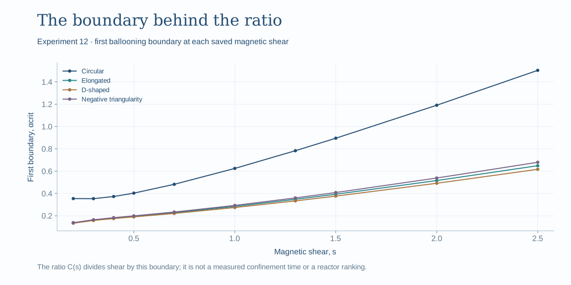
In the shaped Connor–Hastie–Taylor-style model, magnetic shear s describes how field-line pitch changes across the plasma. The normalized pressure-gradient parameter α drives the disturbance. At each saved shear value, the calculation locates the first critical boundary, αcrit, then forms C(s) = s / αcrit.
The ratio rises and flattens across part of the sampled interval, at different levels for different shapes. A larger ratio here means a smaller critical pressure-gradient parameter at fixed shear; it must not be read as “a better reactor.”
| Geometry | κ | δ | Mean C, high-s subset | CoV |
|---|---|---|---|---|
| Circular | 1.0 | 0.0 | 1.656 | 1.71% |
| Elongated | 1.7 | 0.0 | 3.760 | 3.45% |
| D-shaped | 1.7 | 0.33 | 3.932 | 3.90% |
| Negative triangularity | 1.7 | -0.3 | 3.618 | 2.97% |
From a numerical plateau to a mathematical question
A separate saved calculation searches for the maximum of the ratio. Differentiating C(s) = s / αcrit(s) gives a useful check: at an interior stationary point with a differentiable, nonzero boundary, α′crit = αcrit / s. This identity identifies a tangent condition; by itself it proves neither uniqueness nor a global maximum.
| Geometry | Peak shear | Peak C | Saved interval above 98% of peak |
|---|---|---|---|
| Circular | 1.785 | 1.682 | 1.3–2.8 |
| Elongated | 2.034 | 3.877 | 1.5–2.9 |
| D-shaped | 2.121 | 4.072 | 1.6–3.0 |
| Negative triangularity | 1.935 | 3.714 | 1.4–2.8 |
The reported peaks invite a sharper question: under which assumptions on the boundary is there a unique peak, and how sensitive is it to the discretization and geometry model?
Inspect the saved tangent residuals →Equilibrium and external kink: two further steps
Experiment 13 uses FreeGS to solve the Grad–Shafranov equilibrium problem before applying the shaped ballooning diagnostic. This is a different level of modeling from prescribing a shape. Its archived run covers three plasma currents and eight pressure inputs, with 28 sampled locations per case.
| Pressure input (kPa) | 5 MA | 10 MA | 15 MA |
|---|---|---|---|
| 50 | 0 / 28 | 28 / 28 | 28 / 28 |
| 100 | 0 / 28 | 5 / 28 | 28 / 28 |
| 200 | 0 / 28 | 0 / 28 | 7 / 28 |
| 500 | 23 / 28 | 0 / 28 | 0 / 28 |
| 1000 | 28 / 28 | 6 / 28 | 0 / 28 |
| 2000 | 28 / 28 | 23 / 28 | 0 / 28 |
| 3000 | 28 / 28 | 27 / 28 | 18 / 28 |
| 5000 | 28 / 28 | 28 / 28 | 24 / 28 |
Version check: the saved file’s headline says the equilibria remain ballooning-stable past the Troyon limit, but its rows include unstable locations in that range. The table preserves those rows; this artifact is not treated as confirmation of the headline. Reconciliation with the manuscript version remains necessary.
The v5 manuscript also reports an external-kink energy-principle scan across 20 current profiles. In its wall-free limit, it reports a natural-unit ratio βN,crit / li of 0.163 ± 0.004, with 2.4% variation across profiles. That is a reported model result. Its proximity to 1/(2π) does not establish an exact identity or a topological derivation.
CHIHIRO turns the calculations into separate diagnostics
The Rust implementation includes a GEQDSK equilibrium reader, profile extraction, and a combined diagnostic report. Its channels retain different physical questions rather than treating one favorable number as a certificate of plasma stability.
| Channel in the implementation | Question it addresses |
|---|---|
| Ballooning | Does the modeled pressure-driven disturbance become unstable? |
| External kink | Does the modeled global displacement lose stability? |
| Edge localized | What does the edge-mode diagnostic report? |
| Density limit | How does density compare with the chosen limit model? |
| Vertical stability (VDE) | Does the modeled vertical displacement remain restoring? |
| Neoclassical tearing (NTM) | What does the magnetic-island evolution model imply? |
| Resistive wall mode (RWM) | How does the wall/rotation model change the mode margin? |
The implementation also includes Cheeger-cut and spectral calculations, trajectory monitoring, negative-triangularity and spherical-tokamak modules. The next validation step is to compare declared observables with independent codes and discharge records, while checking numerical refinement and model sensitivity.
Follow the work
Bee Rosa Davis · Independent research. The plots here are rebuilt from saved numerical records supplied in the CHIHIRO repository. No plasma solvers or performance benchmarks were rerun for this website update.