HALCYON: canonical lattice and connection geometry
Research settingIndependent
HALCYON has an inspectable computational result: a finite gauge-field simulation on a 60-vertex, 90-edge, 32-face lattice. That record is distinct from the conceptual hardware and the separate mechanical-response illustration.
From the research record
Inspect the work
Original figures, recorded values, and explicit model details. Each exhibit identifies its source and what the comparison means.
The complete saved validation verdict
Scroll horizontally to inspect the full table →
| Check | Recorded verdict |
|---|---|
| Substrate identities | PASS |
| Energy conservation | PASS |
| Covariant Gauss residual | PASS |
| Time reversibility | PASS |
| Migdal-Witten analytical target | PASS |
| Gauge invariance | PASS |
| Microcanonical vs canonical | FAIL |
| Beta-scan | PASS |
| Operational beta envelope | PASS |
| Sector classifier | NOT APPLICABLE |
Run halcyon_dde14a276d54: eight PASS, one FAIL, and one NOT APPLICABLE. In particular, microcanonical versus canonical does not pass. These checks concern the finite simulation and do not establish a hardware effect.
Read the technical figure
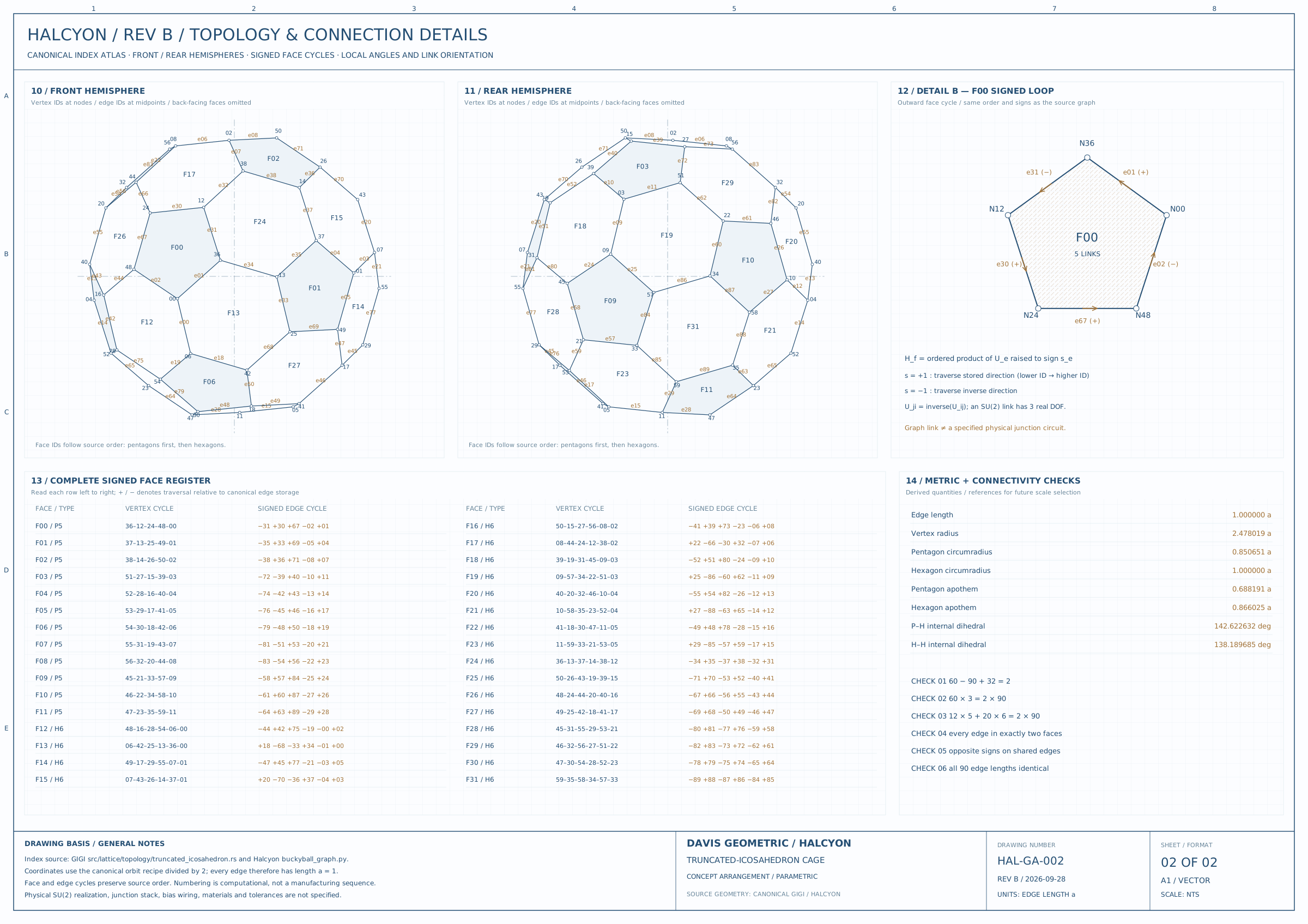
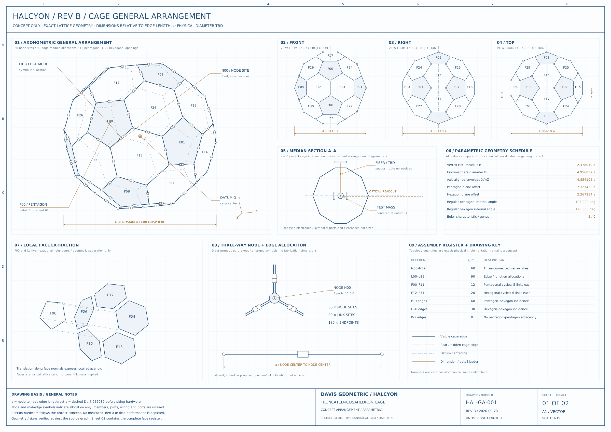
Canonical vertices, oriented edges, face cycles, and connection details from the project engineering sheets. No invented field evolution.
Canonical vertices, oriented edges, face cycles, and connection details from the project engineering sheets. No invented field evolution.
Supporting detail
What the recorded run contains
Run halcyon_dde14a276d54 uses SU(2), coupling β = 2.5, FP64 arithmetic, and second-order leapfrog integration with timestep 0.02 for 1,000 steps. The report records a seed, code commit, library versions, and 50 measurement frames spanning model time 0.4 to 20.0.
The substrate identities are checked explicitly: 60 − 90 + 32 = 2, the summed face perimeters equal 180, and every edge belongs to two faces. These are checks on the constructed finite lattice.
A diagnostic that changed when the correct operator was used
The saved report gives a maximum sampled relative energy change of 4.850 × 10⁻⁵. It also contrasts the covariant Gauss residual with a flat residual on the same state: the final covariant maximum is 4.968 × 10⁻¹⁵, while the flat residual is 0.84252. The distinction is operationally important because the gauge model uses the covariant constraint.
The report explicitly identifies its conjugate-gradient Gauss projection as a global elliptic solve used for validation/restoration. It is not a local physical update. Residuals sampled at measurement frames do not certify unobserved intermediate steps.
Why the mechanical animation is a different model
The nudge demonstration solves a damped, forced oscillator with an inertia ratio selected by the visitor. The field trajectory does not produce that ratio. At 50% assumed inertia, the initial acceleration doubles under the same force because the oscillator equation was given half the inertial mass.
This is a useful explanation of a proposed measurement, but it is not evidence that the gauge configuration changes inertia. The finite simulation also does not establish a continuum Yang–Mills mass gap.
Sources, scope, and next question
Saved June 2026 simulation report and explicit response-model assumptions.
The computational follow-up is trajectory and discretization sensitivity. The hardware follow-up is a separate controlled measurement with a physical coupling model; it cannot be supplied by reinterpreting the oscillator animation.