Geometric pigeonhole: from samples to holonomy
Inspect the covering assignment, the metric proof, the excursion condition, and the reference-frame construction needed for closed-loop holonomy.
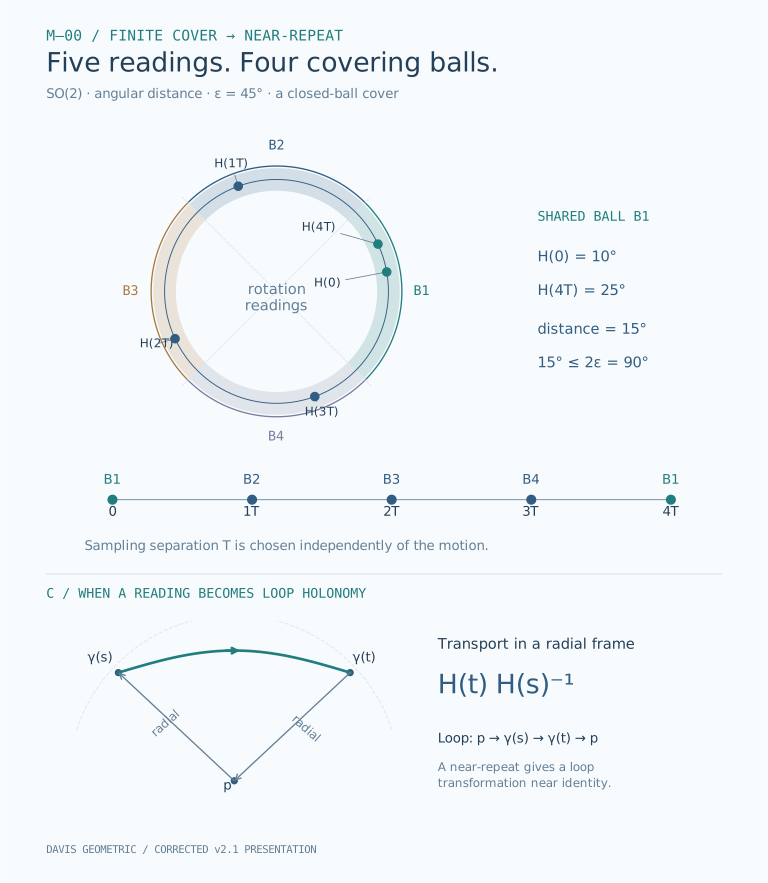
01 / Work through the construction
Read the complete proof and its holonomy interpretation
Theorem A · finite-cover pigeonhole
Let (X, d) be a metric space, ε > 0, and N = NX(ε) < ∞ its ε-covering number. Fix an ordered cover by N radius-ε balls. Let H: [0, L] → X be any map, and prescribe T > 0. No continuity is required.
Proof. The N+1 times tj = jT, j = 0, …, N, all lie in [0, L]. Assign each reading to the first ball containing it. Two readings share a ball. Their distances to its center sum to at most 2ε, while their distinct sampling times differ by at least T. This is the classical pigeonhole principle applied to a finite cover. L* = NT is a sufficient horizon, not a claim about the earliest repeat.
Why a near-repeat is not yet a return
A constant map never leaves home, yet satisfies Theorem A. Under the same setup, Theorem B adds R > 2ε and τ > 0, with an excursion from every starting time: for each s ∈ [0, L−τ], some u ∈ [s, s+τ] satisfies d(H(u), H(s)) > R. If L ≥ Nτ, there exist s < u < t with d(H(s), H(t)) ≤ 2ε and d(H(u), H(s)) > R.
Proof. Apply Theorem A with T = τ and order its two times s < t. The promised excursion fits into [s, s+τ] ⊆ [s, t]. Its distance exceeds R > 2ε, so u is neither s nor t. This supplies the intervening excursion.
Where parallel transport enters
Along a smooth unit-speed path γ on a Riemannian manifold, fix a smooth orthonormal reference frame F(t). Read the parallel-transported initial frame in F(t): H(t) = [Pγ|[0,t]F(0)]F(t). These readings lie in SO(n). Give that group a fixed normalized bi-invariant metric. Its compactness supplies a finite covering number.
H(t) is transport expressed in a frame, rather than itself a closed-loop holonomy. With a radial frame from p, the loop p → γ(s) → γ(t) → p has matrix H(t)H(s)−1 in the frame at p. Bi-invariance gives d(H(s), H(t)) = d(I, H(t)H(s)−1). A near-repeat thus gives a loop holonomy close to the identity. An arbitrary moving frame does not provide that geometric closing path.
What curvature does—and what it does not supply
The connection form ω in F gives H′ = −ω(γ′)H and the Lipschitz bound d(H(s), H(t)) ≤ Λ|s−t|, with Λ = sup ‖ω(γ′)‖. For 0 < Λ < ∞ and T ≤ L, the pair (0, T) already gives a near-repeat whenever T ≤ 2ε/Λ. Above that threshold, this estimate alone no longer suffices. If Λ = 0, the reading is constant.
The source’s radial-frame estimate Λ ≤ C(n)κr₀ is stated under all of these conditions: |K| ≤ κ, γ ⊂ B(p, r₀), r₀ < inj(p), and √κ r₀ ≤ c for a fixed sufficiently small c > 0. See the small-ball definitions. This bounds the rate; it does not force an excursion, determine the earliest return, or establish a horizon proportional to 1/κ. The elementary animation uses Theorem A and does not depend on this geometric estimate.
Source: the supplied v2.1 text, recovered from its untruncated readout in the linked review chat, with the subsequent board corrections incorporated into this presentation. The source snapshot retains its original “v2” heading. Theorem A is a standard finite-cover application of pigeonhole, not a claim of a new counting principle.
02 / A complementary view
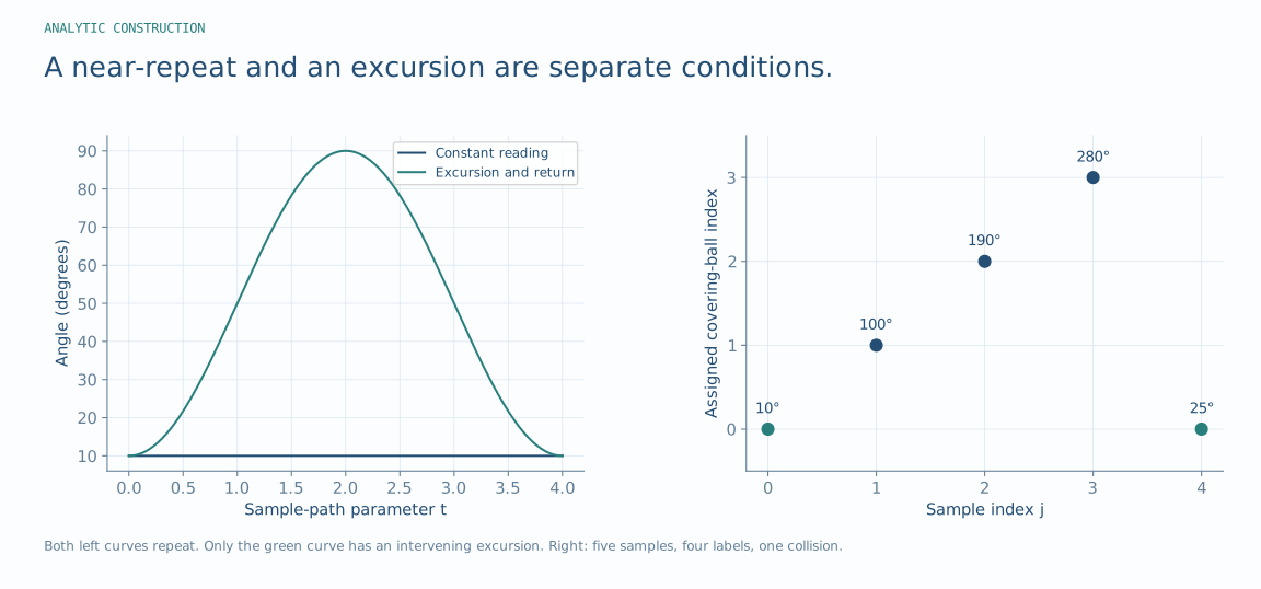
03 / What to check when applying the idea
Identify the state space, the equivalence rule, the distance or observable, and the assumptions used by the argument. Then ask which part is an identity, which part is a model choice, and which part needs an empirical test. The worked constructions illustrate the stated mathematics; they are not evidence that every dataset admits the same geometry.
Use the linked proof review to distinguish the retained conditional statements from the broader manuscript claims requiring correction. Original manuscript titles identify sources and do not override the narrower conclusions on the current research pages.
Sources, versions & further reading
Additional diagnostic plates are analytic constructions or descriptive re-plots of the saved record, as labeled. They do not introduce new experimental validation.