Earth & energy systems / AURORA
AURORA: conservation receipts inside an atmospheric dynamical core
AURORA explores making conservation checks part of the simulation interface. Its specification records what each timestep should preserve and when the solver should refuse to continue.
Research settingNASA
TL;DR
In brief
The question
Can an atmospheric simulation check its own conservation laws at every timestep, and halt rather than continue when a check fails?
What the work does
A v0.1 specification for a shallow-water integrator on the sphere: a four-step Störmer–Verlet scheme with in-step divergence projection, per-step receipts for energy, mass, potential vorticity and circulation, and ten test gates.
What is still open
No completed run of the gates is reported in the reviewed sources. The first milestone is a fifteen-day Williamson Test 2 run with published error norms.
Available recordDynamical-core specification and staged benchmark plan; design targets are not completed benchmark results.
From the research record
Inspect the work
Original figures, recorded values, and explicit model details. Each exhibit identifies its source and what the comparison means.
The staged benchmark ladder
Scroll horizontally to inspect the full table →
| Stage | Named comparison | Question being separated |
|---|---|---|
| Shallow-water core | Williamson cases 2, 5 and 6 | Balanced flow, topography and evolving wave structure |
| Forced dry atmosphere | Held–Suarez | Response to idealized forcing and damping |
| Idealized moist climate | Aquaplanet | Climate behavior under simplified boundary conditions |
| Prescribed surface conditions | Prescribed sea-surface-temperature experiments | Comparison with externally specified boundary forcing |
The named stages come from the companion; the right column is an editorial reading guide. This is a benchmark plan, not a pass/fail table. Conservation receipts and solution error must both be reported when a stage is run.
The research in context
Global weather and climate models are built around a dynamical core: the part that advances wind, pressure and mass on a discretized sphere from one timestep to the next. Every discretization introduces small errors, and over long runs some accumulate as slow drift in quantities the real atmosphere conserves, such as total energy, total mass and potential vorticity (a combination of spin and layer thickness carried by air parcels). Drift is usually measured after a run rather than checked during it. Because forecasts and climate projections depend on long integrations, errors that quietly accumulate in conserved quantities are hard to separate from genuine physical signal.
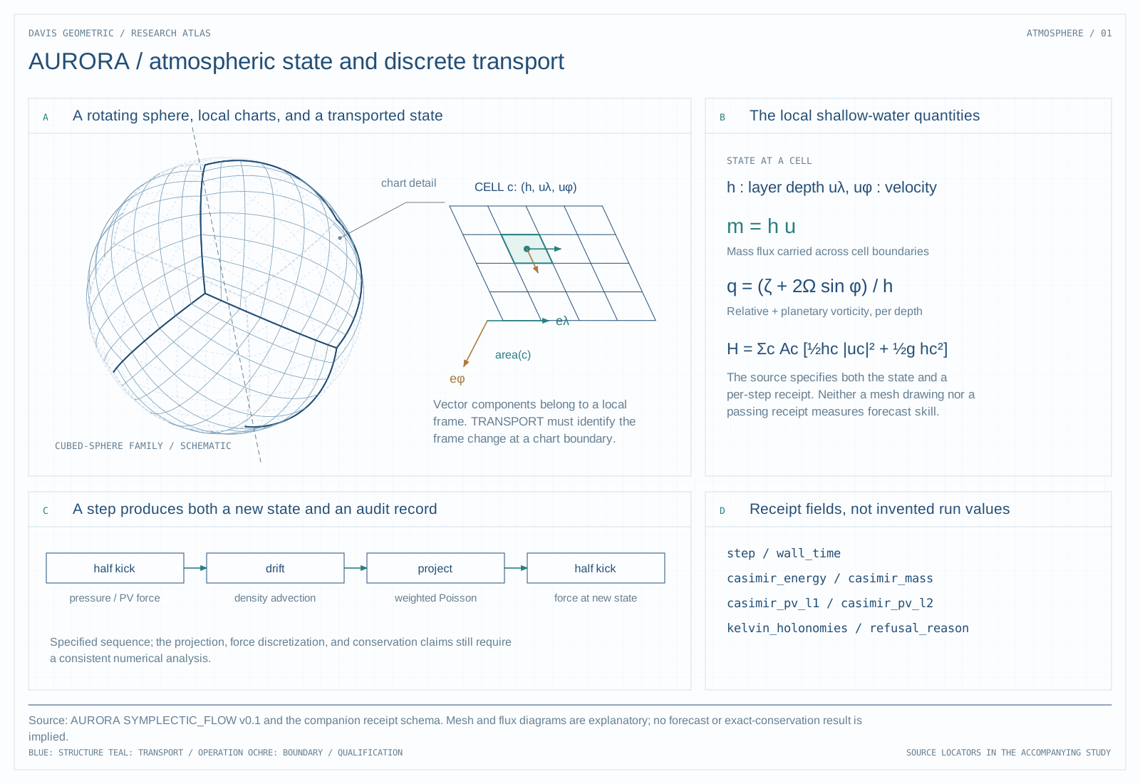
AURORA’s symplectic-flow specification (v0.1, June 2026) restricts itself to the shallow-water equations on a rotating sphere: a single fluid layer described by depth and two velocity components on a cubed-sphere or latitude–longitude mesh. Each step is a leapfrog sequence — a half-step update from pressure gradient and Coriolis force, a full-step advection of depth, a conjugate-gradient projection that removes mass-flux divergence, then a second half-step update. Spatial operators use discrete exterior calculus, in which applying the discrete derivative twice gives exactly zero. The specification reuses the four-step skeleton of the project’s lattice Yang–Mills integrator, changing only the force, advection and projection operators.
The tests are ordered as ten gates, each required before the next: unit checks of the force, of mass conservation in the advection step and of projection convergence; then Williamson Test 2, a steady geostrophic flow with a known exact solution, at a 150-second timestep for one day (576 steps) and fifteen days; then circulation around tagged loops at the equator and 30° north and south; then Williamson Tests 5 and 6. The specification explicitly excludes the three-dimensional core, moisture and clouds, and the regime-classification layer, whose receipt field is fixed at zero in this version.
What a timestep is expected to report
The proposed receipt includes energy, mass, potential-vorticity quantities, selected circulation loops, and a refusal reason when a check fails. The intended benefit is an inspectable account of numerical behavior during the run, rather than a drift statistic reported only after completion.
The design combines discrete geometric operators on a rotating sphere with explicit treatment of coordinate and frame changes. This connects the representation question to a concrete numerical task: the same atmospheric state should not acquire a different physical interpretation because it was expressed in another chart.
The benchmark sequence is part of the research design
The companion names Williamson test cases 2, 5, and 6, followed by Held–Suarez, aquaplanet, and prescribed-sea-surface-temperature experiments. This moves from idealized dynamical-core behavior toward a comparison with observations. Each stage tests a different claim.
The specification’s “8ε” receipt tolerance is a design claim requiring an error analysis for the actual implementation. A symplectic integrator does not generally preserve the original Hamiltonian exactly, and a stable conserved-quantity check alone does not establish accurate waves, circulation, or weather forecasts.
Why conservation is useful but insufficient
A solver can conserve a quantity while propagating a disturbance at the wrong speed. Clouds, forcing, assimilation, and initial-condition uncertainty also affect forecast skill. The representative contribution is the proposed conservation-aware computation and its staged tests, not a claim that a new dynamical core resolves climate uncertainty.
The next research step
Publish the first completed benchmark with its mesh, integrator, timestep, error norms, and receipt history. Compare both conservation and the evolving solution before advancing to a broader forecast claim.
Background mathematics and definitions
Specify a rotating-sphere discretization and the discrete invariants it is intended to respect. Test the algebraic identities independently of time integration. Then measure accumulated integration error and solution accuracy against declared reference problems.
- M
- The declared discrete mass functional.
- Discrete identity
- An exact relationship among specified algebraic operators.
- Forecast skill
- Agreement with observations under a defined prediction task.
Illustrative example
In a two-cell closed system, transferring q from cell A to cell B changes (mA,mB) to (mA−q,mB+q), leaving total mass unchanged. Every q conserves that total, including a physically wrong transfer. Conservation alone cannot choose the correct evolution.
This background example is separate from the source records and the main technical figure.
Source record
Additional source versions reviewed
-
aurora/AURORA_SYMPLECTIC_FLOW_SPEC.mdLocal project manuscript or report · not republished here
No new experiments are reported in this research note. Figure captions distinguish saved research records, source-model calculations, and explanatory diagrams.