Algorithms & computing / GPU / Sudoku
GPU constraint solving: propagation, relaxation, and search
The Sudoku work is a concrete solver architecture: a three-phase CUDA pipeline that combines constraint propagation, a continuous relaxation, and discrete search. Its research question is how to direct parallel effort toward the parts of the constraint graph that can resolve the most remaining choices.
Research settingIndependent
TL;DR
In brief
The question
Can a local priority tell a GPU constraint solver where propagation and branching will resolve the most remaining choices, and does that help on a fixed instance set?
What the work does
A three-phase CUDA Sudoku solver (bitmask propagation, continuous relaxation, prioritized depth-first search) with an instance-routing rule, run on 15-clue extreme puzzles and eleven known hard puzzles on a laptop GPU.
What is still open
An ablation inside the same solver: replace the structural priority with minimum-remaining-values or a plain order, keeping propagation, search, instances and hardware fixed.
Available recordSolver and manuscript described in the Sudoku companion; historical benchmark comparisons require separation.
From the research record
Inspect the work
Original figures, recorded values, and explicit model details. Each exhibit identifies its source and what the comparison means.
Three operations inside the CUDA solver
Scroll horizontally to inspect the full table →
| Phase | Representation | Operation | Output used by the next phase |
|---|---|---|---|
| Propagation | Candidate bitmasks | Arc consistency and hidden singles | Reduced candidate domains |
| Relaxation | Softmax probabilities | Continuous energy relaxation | Candidate preferences |
| Search | Discrete assignments | Iterative-deepening depth-first search | A checked assignment or continued search |
This is the architecture described by the solver companion. It does not reuse the inconsistent historical speedup headline or pool kernel latency with batched throughput.
The research in context
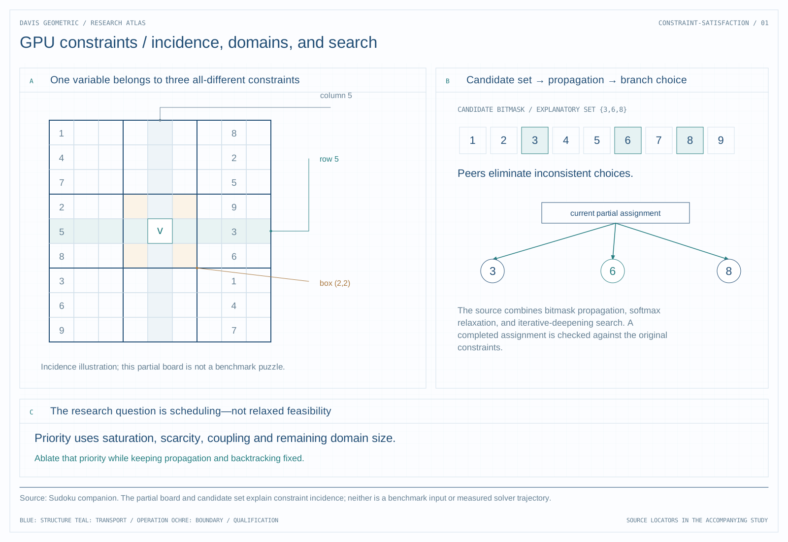
A constraint satisfaction problem asks for values for a set of variables such that every rule holds at once. Sudoku is a compact example: 81 cells, each with up to nine candidate digits, and 27 all-different constraints over rows, columns and boxes. General constraint satisfaction is NP-complete, so practical solvers combine propagation, which deletes candidates that cannot appear in any solution, with search, which guesses a value and backtracks on contradiction. On a GPU the question becomes one of allocation: thousands of threads are available, and a policy must decide which variables to examine and which branches to explore first.
The deposited manuscript (February 2026) and its public repository, sudoky-energy, describe a CUDA solver with an instance-level gate. A parameter Γ, computed from the amount of assigned structure relative to the largest local constraint density, sends an instance to propagation alone (Γ > 1.0), to all three phases (0.35 < Γ ≤ 1.0), or to propagation followed directly by search (Γ ≤ 0.35). The relaxation phase shrinks its step size where local constraint density is high. The search phase orders values by the local priority and prunes branches with a holonomy-based dead-end test. The manuscript states that minimum-remaining-values, the degree heuristic and checkerboarding are recovered when particular weights are set to zero.
The deposit reports runs on 15-clue extreme Sudoku (66 empty cells, Γ ≈ 0.19, so under the gate the relaxation phase is bypassed) on an NVIDIA GeForce RTX 5070 Laptop GPU with CUDA 13.1. A batch of 65,536 instances was fully solved at about 260,000 puzzles per second. For a single instance it reports 20.4 milliseconds of GPU time including host overhead, against 77.8 milliseconds for its Dancing Links implementation. The project page separately reports a 7.8-millisecond average kernel time, excluding transfers, across 11 well-known hard puzzles. These measure different things and are not combined here.
Three kinds of work inside one solver
The first phase uses bitmasks for arc consistency and hidden-single detection. The second represents candidate choices with softmax probabilities and relaxes an energy objective. The third performs iterative-deepening depth-first search with a structural branch priority. These are distinct operations, so their contributions should be measured separately.
The proposed local priority combines saturation, scarcity, and coupling. A variable’s information-value score includes its neighbors’ local scores and divides by its remaining domain size. This makes the mechanism more specific than the claim that geometry makes puzzles easy: it is a computable proposal for choosing where to propagate or branch.
The timing comparisons need different denominators
The companion mixes batched throughput, individual hard-puzzle latency, CUDA kernel timing, and comparisons against Python, Dancing Links, and an energy-based model. Those are different measurements. Kernel timing excludes transfers; a large batch can amortize costs that a single difficult puzzle cannot.
One published headline is internally inconsistent with its nearby latency table: 313 milliseconds divided by 7.8 milliseconds is about 40, not 40,128. This account therefore preserves the solver design without carrying that speedup headline forward. Finding a solution, proving uniqueness, and demonstrating infeasibility also require separate comparisons.
The next research step
The decisive experiment is an ablation within the same solver: keep propagation and backtracking fixed, then replace the structural priority with minimum-remaining-values and a simple unweighted order. That would identify the scheduling contribution.
Background mathematics and definitions
Represent each variable by its finite candidate set and each constraint by the combinations it forbids. Compare a baseline priority with the proposed structural priority while keeping propagation and backtracking identical. A heuristic called curvature needs an explicit computable definition; its name alone does not supply a manifold or a proof of difficulty.
- Dᵢ
- Current candidate set for variable i.
- Propagation
- Removal of values that cannot satisfy a specified local consistency rule.
- Scheduling policy
- The rule choosing which variable or constraint receives work next.
Illustrative example
For three variables constrained to be all different, let A={1}, B={1,2}, and C={2,3}. Propagating A removes 1 from B; propagating the resulting B={2} removes 2 from C. This exact miniature trace explains dependency and available parallelism without predicting GPU speed.
This background example is separate from the source records and the main technical figure.
Source record
- Sudoku project material.
- CSP project material.
- Curvature-Guided Wavefront Execution for GPU-Accelerated Constraint Satisfaction on the Davis Manifold.
No new experiments are reported in this research note. Figure captions distinguish saved research records, source-model calculations, and explanatory diagrams.