Weak connections between groups
Small weights on the brown links · slower exchange- Reached the other group
- 1.4%
- Still at the starting node
- 18.0%
- Spectral gap λ₁
- 0.0071
Spectral geometry / Transformer attention
A network can hide its organization in thousands of connections. A heat kernel asks a simpler question: if a pulse starts here, where can it spread—and what slows it down?
A language model builds an answer by repeatedly combining information from its context. My research asks how those connections are organized: which token positions stay closely coupled, which groups exchange information easily, and how that organization changes across layers and attention heads.
The question behind the picture
Consider: “The key to the cabinets is missing.” The verb agrees with key, even though cabinets is closer. A useful representation has to preserve relationships that are not obvious from word order alone.
Attention is one way a transformer combines context: each head forms a weighted mixture of information from token positions. Those weights make a network. The heat kernel lets me inspect the organization of that network without having to read thousands of weights one at a time.
The illustration below isolates one question: does a network mostly keep information within local groups, or does it readily connect those groups? It uses constructed graphs so the mechanism is easy to see; the recorded language-model measurements come later.
Start here / What is a heat kernel?
Touch one spot on a metal plate with something hot. At first, the heat stays near that spot. Over time it spreads. The plate’s shape and its ability to conduct heat determine where it goes.
A heat kernel describes the response to that tiny, concentrated starting pulse. It tells you how much of the response appears at each destination after a chosen amount of time. Repeat that question for every possible starting spot, and you have a complete map of how the system spreads a disturbance.
On this page, the plate becomes a network. The lines conduct a mathematical pulse between dots. Strong and weak connections leave different patterns, making the network’s organization visible.
For a finite graph, choose a positive-semidefinite Laplacian L. The diffusion equation is du/dt = −Lu, with initial state u(0) = u₀. Its solution is u(t) = K(t)u₀, where K(t) = exp(−tL) is the heat-kernel matrix. The exponential is a matrix exponential, not an entry-by-entry operation.
With column-vector states, Kᵢⱼ(t) is the response at position i to a unit impulse initially placed at position j. At t = 0, K(0) = I: nothing has spread yet. The identity K(t + s) = K(t)K(s) means that diffusing for s and then t is equivalent to diffusing for their sum.
In this study, A contains attention weights, W = (A + Aᵀ)/2 makes them symmetric, and D is diagonal with Dᵢᵢ = ΣⱼWᵢⱼ. For positive degrees, the symmetric normalized Laplacian is L = I − D⁻½WD⁻½. If Lφₖ = λₖφₖ with orthonormal eigenvectors, then Kᵢⱼ(t) = Σₖ exp(−tλₖ)φₖ(i)φₖ(j). Large-eigenvalue modes fade quickly; small-eigenvalue modes persist. This is the link between the animation and spectral geometry.
The normalized symmetric kernel does not generally have columns summing to one. To display a conserved probability pulse, this companion uses P(t) = D½K(t)D⁻½. Thus the displayed percentage at i for a pulse starting at j is 100 × Pᵢⱼ(t). P and K have the same diagonal and trace. The two constructed graphs have positive degrees even when the connections between their groups are removed.
On a Riemannian manifold, the analogous kernel Hₜ(x,y) solves the heat equation for the chosen Laplace–Beltrami operator and boundary conditions: u(t,x) = ∫ Hₜ(x,y)u₀(y) dvol(y). The graph uses a finite sum in place of the integral. Its relationship to a continuous geometry depends on how the graph and operator are constructed.
See how the study builds this operator from attention ↓ · Read the paper’s mathematical formulation
01 / Same starting point · same clock · different connections
In a language model, attention connects token positions—words or parts of words. Here, each dot stands for a position, and each line is a weighted connection. The two clusters are groups of positions that are strongly connected within themselves. The brown lines between the groups are the “bridges.” They represent weaker or stronger coupling between groups in a symmetric view of attention.
On the left, those links have low weights: a test pulse spreads within its starting group before much reaches the other group. On the right, the same links have higher weights, so the groups exchange the pulse sooner. Watch the “Reached the other group” percentage to see the difference. This is a controlled illustration of connectivity, not a recording of words moving through an LLM.
An analysis scale, not elapsed inference time. One unit of pulse is conserved in each graph.
The nearby group fills first. Weak connections between groups delay the exchange between groups.
Reading this as an attention pattern: the left graph keeps the two token groups more separate at this scale. The right graph allows faster exchange between them. In a model, that distinction could matter when an answer needs a relationship spanning both groups.
Constructed graphs, not recorded transformer attention. Color and node size show pulse probability on a shared scale. Moving dots indicate net diffusion direction; they are not tokens traveling through a model. Crossing lines do not create extra nodes.
02 / A different view of the same calculation
Read one column from top to bottom: it shows where a pulse from that starting node ends up. Near time zero, the bright diagonal means each pulse stays where it began. Later, bright square blocks reveal groups that exchange mostly with themselves. Broader color across the blocks shows exchange between groups.
Weak connections between groups
A network has characteristic patterns of variation, called modes. Diffusion smooths out the fast ones first. Slow modes describe differences that persist, such as one group remaining more concentrated than another. The heat trace adds their remaining weights into one curve.
At t = 0 the trace is 18. In the long-time limit it approaches 1 for a connected graph, or 2 when the two groups are disconnected. The finite right edge of the plot is not that limit.
The spectral gap describes the slowest nonconstant mode’s decay rate. The narrow-bridge graph has a smaller gap: the difference between its two groups takes longer to disappear. Applied to attention, this gives a measurable description of integration and separation. Neither is automatically better—local processing may benefit from separation, while a task requiring a distant relationship may need stronger exchange.
03 / From language to a graph
Here, cognition means how a model organizes and transforms contextual information while producing a continuation. Attention patterns offer one observable part of that process. A heat kernel turns those patterns into questions we can compare across prompts, layers and heads.
A node represents a token position—a word or part of a word. For one head in one layer, the attention weights describe how that position mixes information from the available context. A different prompt can produce a different graph.
The study makes an undirected view of those weighted connections and constructs a normalized Laplacian: an operator describing how differences across connected positions can smooth out. Its spectrum tells us which patterns fade quickly and which persist.
Short diffusion times emphasize nearby relationships. Longer times reveal how groups connect to the wider context. Comparing these profiles across layers can show how the organization of attention changes as token representations are updated.
This suggests concrete research questions. Does a head mostly bind a small group of positions? Does another connect those groups? Does a prompt requiring a distant relationship change that pattern? These are hypotheses about computational roles that can be tested by changing or removing the head and checking the output.
The analysis uses a symmetric view of attention, so it discards direction. Attention weights also omit the content of value vectors, feed-forward computations and residual updates. The diffusion picture is a probe of one part of the model, not a replay of its complete computation.
The symmetric normalized kernel K is not generally a probability-transition matrix. This page displays P(t) = D½ K(t) D⁻½, so each column sums to one. Its diagonal and trace equal those of K. This keeps the pulse conserved while using the paper’s normalized Laplacian and spectrum.
For each graph, all 18 eigenpairs are retained. Independent matrix-exponential checks verify the spectral calculation, positivity, mass conservation and the disconnected case. At equilibrium, probability is proportional to node degree; it need not be uniform.
04 / A practical research question
A transformer uses many attention heads in parallel. If you want a smaller model, you need to decide which ones to keep. A head can have large or variable attention weights without providing a distinctive pattern of connectivity.
Two heads can have very different-looking weight matrices yet organize connections in similar ways. Conversely, a small set of weights may provide the only strong link between two groups. Heat-kernel profiles offer a way to compare these patterns across scales, rather than rank a head only by how large or variable its weights are.
The next step is an intervention: mask the selected heads, run the model, and measure what changed. Similar descriptors alone do not prove that two heads are interchangeable.
The useful output is a testable comparison: identify a geometric difference, intervene on the component, and check whether the difference matters for model performance.
05 / Security implications · A proposed extension
You ask an assistant to summarize a document. Inside the document, someone has inserted instructions telling it to abandon your request. The security question is simple: can the assistant read those words without treating them as orders? This is the trust boundary that prompt injection tries to cross.
A model has to attend to a document to summarize it. Strong connections to its words are therefore expected—even when the document discusses an attack. Attention alone cannot tell us whether the model has confused source material with an authorized instruction.
My security question is whether changes in the geometry of attention help distinguish ordinary reading from a successful redirection. We could compare the same task with a clean document, an injected version, and a harmless quotation of the same instruction.
Label token spans by their source: task instruction, retrieved document and generated response. Compare diffusion profiles across heads and layers to find where the relationships change. Keep these labels: a heat trace alone loses the identity of the positions involved.
Compare successful attacks with resisted attacks and benign examples. Test selected heads through controlled interventions. A changed spectral gap becomes useful only if it helps explain or predict the behavior we care about.
Evaluate on unseen documents, attack styles and models. Report missed attacks, false alarms on legitimate work and the cost of monitoring. Include attackers that adapt to the proposed detector.
The potential benefit: an internal signal that helps investigators locate a failure, or helps a monitoring system decide when to pause an action for review. This requires access to model attention, which many hosted APIs do not expose. Any resulting monitor would complement tool permissions and data-access controls; a geometric score cannot grant authority.
There is precedent for investigating attention in this setting: Hung and colleagues’ Attention Tracker (NAACL 2025) studies shifts toward injected instructions. It is a different method, and its results do not validate a heat-kernel detector. Anthropic’s browser-agent research also illustrates why defenses must be tested against adaptive attacks.
Research direction for this companion. The deposited study does not establish prompt-injection detection, attack attribution or prevention of data theft. No attack-detection performance is measured by the animation above.
06 / From the recorded study
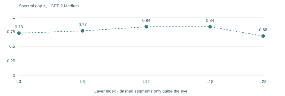
Table 4 reports a larger spectral gap in the middle of GPT-2 Medium than at its entry and exit. In the corresponding diffusion analysis, a larger gap means the slowest nonconstant mode fades faster. This motivates a question about the model: are middle layers organizing context differently from the layers that receive and finish the representation? The profile identifies where to investigate; interventions are needed to establish what those layers do.
The prompt experiment asks a different question: does attention organize itself differently for familiar facts and invented subjects? Compare “The capital of France is” with “The capital of Zorblania is.” The first refers to something real; the second invents an entity. The study compares three prompts of each kind per model.
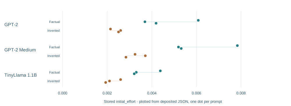
Each dot below is a saved initial_effort value: a summary of how uneven a short-scale heat-kernel signal is across token positions early in generation. The name is the paper’s; the number is a geometric descriptor, not a measurement of mental effort.
The factual prompts have larger values in these saved cases: their short-scale diffusion signatures are more uneven by this descriptor. That supports investigating whether familiar and invented subjects elicit different attention organization. It does not yet identify the cause of that difference or show that a generated answer is correct.
All 36 saved records—including forced correct and incorrect completions—received the same PATTERN_MATCHING classification. The useful next step is to test whether a richer profile predicts behavior on held-out prompts, while controlling wording, tokenization and sequence length.
| Source model | Prompt | Category | Initial effort |
|---|---|---|---|
| GPT-2 | The capital of France is | Factual | 0.006083 |
| GPT-2 | The chemical symbol for water is | Factual | 0.003692 |
| GPT-2 | The speed of light is approximately | Factual | 0.004192 |
| GPT-2 | The capital of Zorblania is | Invented entity | 0.002148 |
| GPT-2 | The chemical symbol for magicium is | Invented entity | 0.002603 |
| GPT-2 | The flobnax constant is approximately | Invented entity | 0.002508 |
| GPT-2 Medium | The capital of France is | Factual | 0.007835 |
| GPT-2 Medium | The chemical symbol for water is | Factual | 0.005195 |
| GPT-2 Medium | The speed of light is approximately | Factual | 0.005319 |
| GPT-2 Medium | The capital of Zorblania is | Invented entity | 0.003249 |
| GPT-2 Medium | The chemical symbol for magicium is | Invented entity | 0.003710 |
| GPT-2 Medium | The flobnax constant is approximately | Invented entity | 0.002841 |
| TinyLlama 1.1B | The capital of France is | Factual | 0.004382 |
| TinyLlama 1.1B | The chemical symbol for water is | Factual | 0.003305 |
| TinyLlama 1.1B | The speed of light is approximately | Factual | 0.003213 |
| TinyLlama 1.1B | The capital of Zorblania is | Invented entity | 0.002601 |
| TinyLlama 1.1B | The chemical symbol for magicium is | Invented entity | 0.002104 |
| TinyLlama 1.1B | The flobnax constant is approximately | Invented entity | 0.001931 |
Model names follow the deposit filenames: the records themselves use “gpt2” in the model field in all three files. Table 9’s reported means align with the TinyLlama file rather than the GPT-2 file named in its caption. This chart uses the individual deposited values and file identities.
The local validation script computes a scaled variance of the heat-kernel diagonal at t = 0.1, then summarizes an early window of the generation trajectory. This “effort” descriptor is not an energy measurement or a direct observation of retrieval. Prompt wording, tokenization and sequence length remain possible confounds.
08 / What this lens establishes
For the defined graph, the kernel, spectrum and diffusion behavior are determined by its weights. The companion’s graphs and calculations are reproducible.
The paper reports attention profiles and a pruning comparison in GPT-2-family models, plus small prompt studies in GPT-2 and TinyLlama. The graphs above are teaching examples, separate from those records.
Test whether descriptors predict the effect of removing a head on held-out tasks, across seeds and model families. Prediction needs that comparison; a striking heat map alone cannot establish it.
The heat trace is a spectral descriptor, not a unique identity: different graphs can share a spectrum. The paper’s curvature quantities should likewise be read as experimental proxies, not automatically as a manifold’s scalar curvature.
For a finite graph, K(t) = I − tL + O(t²), so the literal limit 6 ∂ₜ log Kᵢᵢ(t) at zero equals −6Lᵢᵢ. It does not by itself extract the scalar-curvature term in a manifold heat-kernel expansion. The local validation code uses the different diagonal-variance descriptor described above.
Davis, B. R. (2025). Spectral Geometry of Transformer Cognition: Heat Kernel Analysis Reveals Functional Organization in Language Models. Zenodo, v1. Published December 2, 2025.