Engineering systems / FAL-CORE / The Geometry of Flight
FAL-CORE: one flight model, eight views of control and adaptation
FAL-CORE connects state-space modeling, optimal control, estimation, and adaptation through an interactive aerospace example. The implementation follows an F-16 longitudinal model through eight lessons, using bicycle analogies to make the control questions accessible.
Research settingMach Industries
TL;DR
In brief
The question
Can one aircraft pitch model, carried through eight lessons, make the assumptions behind fixed and adaptive flight controllers visible and comparable?
What the work does
An interactive application with hand-written numerical routines: an F-16 short-period plant plus elevator actuator, analyzed through frequency response, LQR, Kalman estimation, Lyapunov design, model-reference adaptation and four update laws.
What is still open
Which stability conditions are proved for the implemented update laws, and how the four laws compare under declared disturbances, actuator limits and realistic model mismatch.
Available recordInteractive models developed with Mach Industries; source contains eight lesson modules and a four-state augmented plant.
From the research record
Inspect the work
Original figures, recorded values, and explicit model details. Each exhibit identifies its source and what the comparison means.
The actual four-state plant
Scroll horizontally to inspect the full table →
| State derivative | α coefficient | q coefficient | δe coefficient | δ̇e coefficient | Command u coefficient |
|---|---|---|---|---|---|
| α̇ | -1.01887 | 0.90506 | -0.00215 | 0 | 0 |
| q̇ | 0.82225 | -1.07741 | -0.17555 | 0 | 0 |
| δ̇e | 0 | 0 | 0 | 1 | 0 |
| δ̈e | 0 | 0 | -2500 | -70 | 2500 |
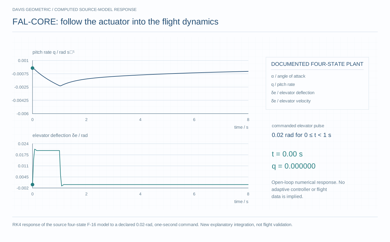
ẋ = Ax + Bu; x = [α, q, δe, δ̇e]ᵀ and y = q. Angle of attack and elevator angle are in radians; q and δ̇e are in rad/s. Coefficients have the corresponding derivative/state units. This is the implemented short-period aircraft model with an elevator actuator, not a propulsion model or a measured aircraft response.
How the actuator enters the model
Scroll horizontally to inspect the full table →
| Element | Source value / equation | Role |
|---|---|---|
| Natural frequency | ωn = 50 rad/s | Sets actuator response scale |
| Damping ratio | ζ = 0.7 | Sets damping of the second-order actuator |
| Actuator equation | δ̈e + 70δ̇e + 2500δe = 2500u | Maps commanded elevator to actual elevator |
| Measurement | C = [0, 1, 0, 0]; D = 0 | Only pitch rate is returned as y |
| Source operating point | Mach 0.6; altitude 15,000 ft | Operating point stated in the source comment |
The operating point is attributed to the model source; its agreement with a particular airframe is not independently established here. The numerical response above uses these same coefficients.
The research in context
Flight control turns a pilot's or autopilot's command into control-surface motion that keeps an aircraft stable and responsive. Engineers describe the aircraft with a state-space model: a few variables, such as angle of attack (the wing's angle to the oncoming air) and pitch rate, whose rates of change depend linearly on the state and the control input. Standard tools ask different questions of that one model: how it responds at each frequency, which gains minimize a stated cost, how to estimate unmeasured states, and how to keep tracking when the model is wrong. Adaptive control, which adjusts its gains during operation, is where those questions are hardest to keep apart.
FAL-CORE is a browser application built with React and Vite. Its numerical routines (linear algebra, complex arithmetic, frequency response, stability margins, Riccati-based LQR design and time simulation) are written by hand in a small library rather than imported, so that the mathematics stays readable as part of each lesson. The plant uses the Stevens and Lewis short-period coefficients for an F-16 trimmed in level flight at Mach 0.6 and 15,000 ft, stacked with a second-order elevator actuator with natural frequency 50 and damping ratio 0.7. Each of the eight modules opens with a bicycle analogy, then gives a geometric reading and the textbook name. A ninth integration module is listed but not yet built.
The adaptation lesson separates tracking from learning. With a square-wave reference that excites the dynamics sufficiently (persistent excitation), the estimated feedback gains approach the values implied by the LQR design. With a constant reference, the same controller still drives tracking error down, but the gains come to rest at different, history-dependent values. A sweep of the adaptation rate at 2, 12 and 80 shows faster gain convergence bought with a larger transient burst in the control signal. The following lesson adds a matched disturbance and compares the plain update with sigma modification, projection onto a norm bound, and a dead zone.
Keep the plant recognizable as the mathematics changes
The source defines a two-state short-period plant with angle of attack and pitch rate, then adds a second-order elevator actuator. The augmented state contains angle of attack, pitch rate, elevator deflection, and elevator velocity. Commanded elevator is the input and pitch rate is the measured output.
Using the same plant throughout is the organizing contribution. A coordinate change, a frequency response, an LQR design, and an observer can be read as different questions about a shared object rather than disconnected equations. The library exposes its matrices and numerical routines to inspection.
From a fixed controller to learning online
The implemented lesson sequence covers linear systems, Bode response, LQR and Riccati equations, robust synthesis, observers and Kalman filtering, Lyapunov analysis, state-feedback model-reference adaptation, and robust adaptive laws. The earlier README describes only a first-lesson prototype; the current source contains all eight modules.
The model-reference adaptation lesson evolves estimated feedback and reference gains while tracking a reference model built from the LQR design. The next lesson compares a plain update with sigma modification, projection, and a dead zone under a matched disturbance. Those choices alter parameter growth and tracking behavior in different ways.
What the interactive comparisons establish
The demonstrations make the implemented update laws and their trajectories inspectable. A plot of decreasing tracking error is not by itself a proof of a claimed Lyapunov argument; the chosen matrix, matching assumptions, disturbance class, and numerical discretization must agree with that argument.
The companion concerns flight-control models. Although the catalog previously grouped it under propulsion, the reviewed source does not establish a measured propulsion improvement. The controller experiments are the more accurate representative work.
The next research step
A useful next report would compare the four adaptive updates on the same declared disturbance and actuator constraints, retaining gain trajectories as well as tracking error. It should state which stability conditions are proved and which behavior is only observed in the numerical example.
Background mathematics and definitions
Declare the simulated plant, parameter uncertainty, measured outputs, update law, and actuator limits. Compare adaptive and fixed controllers under the same reference commands and disturbances. State which flight dynamics and actuator behavior are modeled rather than measured.
- Plant
- The flight dynamics and actuator model specified in the experiment.
- Adaptation rule
- The stated online parameter or policy update.
- Saturation
- A physical or simulated limit on the available control input.
Illustrative example
For a toy plant y=gu, reducing an unknown gain g from 1 to 0.5 halves output under the same input. Doubling u could restore output only if the actuator permits it. The example separates parameter adaptation from feasibility under limits.
This background example is separate from the source records and the main technical figure.
Source record
Additional source versions reviewed
-
fal-core/README.mdLocal project manuscript or report · not republished here -
fal-core/src/pages/Home.jsxLocal project manuscript or report · not republished here -
fal-core/src/lib/f16.jsLocal project manuscript or report · not republished here -
fal-core/src/pages/S7_LearningTheBike.jsxLocal project manuscript or report · not republished here -
fal-core/src/pages/S8_PotholeMidLearn.jsxLocal project manuscript or report · not republished here
No new experiments are reported in this research note. Figure captions distinguish saved research records, source-model calculations, and explanatory diagrams.