A · Wings drawn in

Extension 0.62 × Projection 0.0346
A bird changes its shape. The air responds to the new surface. The next movement depends on that response. Follow one point on a crane’s wing from a visible motion to the mathematics that connects the body and the air.
How the work began
“After graduate school, and after government cuts ended my work at NASA, I was working as a waitress when I met Dr. Ryan Rapetti’s wife. I told her about my work as a mathematician at NASA, and she introduced us.
That introduction grew into nearly a year of correspondence—ideas, studies, and challenges. Ryan introduced me to the classical concepts of guidance, navigation, and control; I brought my computational analysis methods and engineering experience to the questions we explored together.
I began recording the experiments in a blog. As the work grew, those notes became a book: The Geometry of Flight, which you can read here for free.”

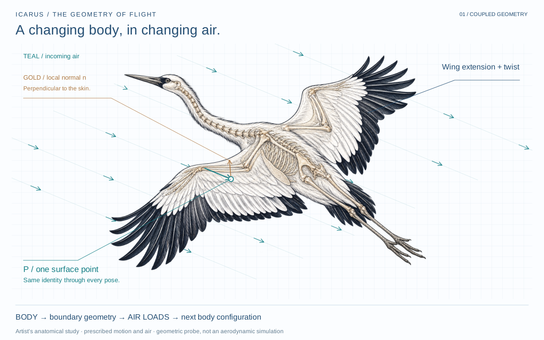
The wings extend and twist; the same surface point moves.
01 / Body bundle
The blue shape is one configuration of the same body. Point P remains on the same patch of skin.
02 / Aerodynamic bundle
At that same P, attach the local air, pressure and shear. Here, the teal air direction is prescribed.
03 / Shared geometry
The dot product compares air and surface directions in one frame. It changes when either changes.
Imagine placing a tiny ink dot, P, on a wing. The bird can extend that wing, twist it, or bank its whole body. P moves in space, but it remains the same material point. This distinction between which point it is and where it is now is the starting point of the book’s body bundle.
Call the reference surface Σ. A configuration assigns a three-dimensional position φ(P) to each point P of Σ. In the book’s notation, the body bundle is Σ × ℝ³ → Σ: over every point of the reference surface, keep the possible position vectors. A section selects one vector for each point. A physically admissible shape needs additional conditions, such as smoothness, no self-intersection, and anatomical or mechanical limits.
The second description attaches the local aerodynamic state to that same P: pressure p, tangential shear τ, and relative airflow u. Pressure is a scalar; shear lies in the local tangent plane; airflow is a vector. These are different kinds of data. A shared geometric language keeps their locations, frames and transformation rules connected instead of treating them as interchangeable numbers.
The dot does not move to a different identity when the wing opens. What changes is its position, its neighboring surface geometry, and the air’s relationship to that geometry. That is the relationship the animation is designed to make inspectable.
The body’s configuration supplies a boundary for an aerodynamic problem. Together with the incoming flow, fluid properties, motion and relevant history, it constrains the fluid solution. That solution supplies pressures and shear stresses on the body. Integrating those stresses over the surface gives a total force and a total moment.
Here n is the outward unit normal and dA is a small area of the deformed surface. The moment uses the distance from the chosen center of mass as a lever arm. The pair (F, M) is called a wrench. These equations describe accounting across a surface; they do not supply the pressure or shear values by themselves.
Section 4.1 abbreviates the coupling as N: Γbody → Γaero. Read this with the flow conditions and modeling assumptions held fixed. Shape alone cannot determine an unsteady fluid state independently of velocity, boundary conditions and history. A numerical aerodynamic model, or appropriate measurements, is needed to evaluate the coupling in an actual application.
The controller then faces an inverse question: among the configurations and actuator settings available to this body, which can produce the required force and moment? The same surface coordinates make the forward calculation and this selection problem part of one connected description.
This illustration implements a small geometric experiment. Its artist-drawn crane is carried by a continuous deformation surface with prescribed extension, twist and bank. The anatomical artwork is illustrative; the deformation model is not a measured bird reconstruction. A fixed material coordinate identifies P. The renderer computes P’s position and two local tangent directions from the surface; their cross product supplies a unit normal n. The same normal drives the gold arrow and the numerical readout.
Material point P / a controlled comparison
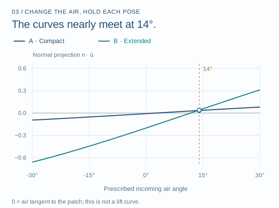
Keep the incoming air fixed at 14°. Extend and reshape the wing. The gold normal turns by 72.7°, but its projection—the part pointing along the teal air direction—barely changes. A single number does not describe the whole relationship.
A · Wings drawn in
Extension 0.62 × Projection 0.0346
B · Wings extended

Extension 1.00 × Projection 0.0400
| Quantity | A · Compact | B · Extended |
|---|---|---|
| Air angle | 14° | 14° |
| Wing extension | 0.62 × | 1.00 × |
| Fold / twist | 28° / 2° | -8° / 18° |
| Bank | -10° | -10° |
| Unit normal n | (−0.008, 0.985, 0.175) | (−0.201, 0.128, 0.971) |
| Projection n · û | 0.0346 | 0.0400 |
The grid follows the same material coordinates around P in both poses. Gold is the unit surface normal; teal is the prescribed unit air direction. Both vectors use the same world frame.
| Step | What is prescribed | What the geometry computes |
|---|---|---|
| 1. Glide | Reference posture and horizontal incoming air | Point position, tangent plane and unit normal |
| 2. Air changes | Air direction tilts; posture stays fixed | The normal projection changes while P and n stay fixed |
| 3. Wings respond | Extension and twist increase; air direction stays fixed | P and n move, changing their relation to that same air |
| 4. Bank | The body rotates and the illustrated air angle changes | Positions and normals are compared in the same world frame |
With both vectors normalized, n · û = cos θ lies between −1 and 1. Zero means the air direction is tangent to the local surface. Magnitude one means it is normal to the surface; the sign distinguishes the two sides. This is enough to demonstrate that changing the body or changing the air changes their geometric relationship. It is not enough to infer lift, drag, stall, stability, or an optimal posture.
All coordinates are dimensionless drawing coordinates divided by 100 for display. “Reference” means the authored full extension, not a measured species wingspan. The animation is a prescribed explanatory sequence, not a controller discovering a response. The entire calculation is available in the geometry source.
The crane makes a large configuration space visible: it can change wing extension, twist, feathers and whole-body orientation. A rigid airframe cannot do all of that. Its configuration and control inputs are limited by its construction. Chapter 4 uses this contrast to ask the same question across platforms: how does the body’s available authority relate to the motion being requested?
Chapter 5 makes another coupling explicit on a quadcopter: position control can demand a world-frame acceleration that the current attitude cannot immediately produce. Reorientation takes time. Representing the request and the available thrust in connected frames exposes that mismatch; a shared representation does not erase inertia, actuator limits or observation delay.
The manuscript’s ICARUS proposal uses geometric state descriptions and an obstruction-dependent modulation of controller gain. Its operational confidence, C = 1/(1 + κ̂), is a defined design quantity, not a calibrated probability of safety. The crane demonstration does not implement or validate that controller. The saved advisory study separately documents the scenario, sampling check and ablations already shown on this site.
“Flight envelope” means the set of states and conditions in which the modeled vehicle can operate subject to its constraints. It is not the visible set of air arrows around the crane. Those arrows show prescribed incident air only; neither a flight envelope nor a CFD flow field has been solved here.
ICARUS asks how a body can respond to its conditions. The accompanying perception idea asks where another moving object could be, given observations and physical constraints. Its output is a set of possibilities under a model, not knowledge of a unique future trajectory.
With the same current state and bounded maneuvering capability, a shorter remaining time allows less additional deviation. But uncertain observations, changing assumptions and new disturbances can widen the estimated set. Proximity alone does not guarantee certainty. This conceptual distinction belongs alongside the body–air explanation, rather than being drawn as if it were the same mechanism.
This study is based on Bee Rosa Davis’s The Geometry of Flight, particularly §4.1–4.4 (body and aerodynamic bundles) and chapter 5 (position–attitude coupling). The supplied preview file includes these chapters. The local author manuscript is the source of the research formulation; this page does not present it as independently reviewed.
The technical excerpt preserves the source discussion of the two bundles and the surface-force equations. The site distinguishes an embedding from an immersion, describes aerodynamic fibers pointwise, and makes the flow conditions behind the coupling explicit. These qualifications matter when translating a geometric description into a numerical model.
A performance claim requires a specified vehicle, identified dynamics, control constraints, sensing assumptions and comparisons against appropriate controllers. Useful evaluation would include tracking error, control effort, constraint violations, failure cases and sensitivity to model mismatch. Neither this explanatory crane nor the shared bundle vocabulary establishes that all classical GNC dead zones have been eliminated.
From the experiments to the book
Follow the correspondence, concepts and experiments into the full manuscript. Read the book here for free, browse its contents, or find the pages behind a question.
587 PDF pages · Supplied author preview · Curvature, Adaptation, and Stability